大数据分析 – 统计方法
大数据分析 – 统计方法
在分析数据时,可以采用统计方法。执行基本分析所需的基本工具是 –
- 相关分析
- 方差分析
- 假设检验
处理大型数据集时,不会出现问题,因为这些方法的计算量并不大,相关分析除外。在这种情况下,总是可以取样并且结果应该是可靠的。
相关分析
相关分析旨在找出数值变量之间的线性关系。这可以在不同的情况下使用。一个常见的用途是探索性数据分析,在本书的 16.0.2 节中有一个这种方法的基本示例。首先,上述示例中使用的相关度量基于Pearson 系数。然而,还有另一个有趣的相关性指标不受异常值影响。该指标称为斯皮尔曼相关性。
的Spearman相关度量是更稳健的对异常值比Pearson法的存在,并给出数值变量之间的线性关系的更好的估计,当数据不是正态分布。
library(ggplot2)
# Select variables that are interesting to compare pearson and spearman
correlation methods.
x = diamonds[, c('x', 'y', 'z', 'price')]
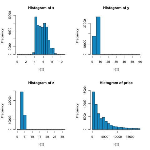
# From the histograms we can expect differences in the correlations of both
metrics.
# In this case as the variables are clearly not normally distributed, the
spearman correlation
# is a better estimate of the linear relation among numeric variables.
par(mfrow = c(2,2))
colnm = names(x)
for(i in 1:4) {
hist(x[[i]], col = 'deepskyblue3', main = sprintf('Histogram of %s', colnm[i]))
}
par(mfrow = c(1,1))
从下图中的直方图,我们可以预期两个指标的相关性存在差异。在这种情况下,由于变量显然不是正态分布的,spearman 相关性是对数值变量之间线性关系的更好估计。
为了计算 R 中的相关性,打开包含此代码部分的文件bda/part2/statistical_methods/correlation/correlation.R。
## Correlation Matrix - Pearson and spearman
cor_pearson <- cor(x, method = 'pearson')
cor_spearman <- cor(x, method = 'spearman')

### Pearson Correlation
print(cor_pearson)
#            x          y          z        price
# x      1.0000000  0.9747015  0.9707718  0.8844352
# y      0.9747015  1.0000000  0.9520057  0.8654209
# z      0.9707718  0.9520057  1.0000000  0.8612494
# price  0.8844352  0.8654209  0.8612494  1.0000000

### Spearman Correlation
print(cor_spearman)
#              x          y          z      price
# x      1.0000000  0.9978949  0.9873553  0.9631961
# y      0.9978949  1.0000000  0.9870675  0.9627188
# z      0.9873553  0.9870675  1.0000000  0.9572323
# price  0.9631961  0.9627188  0.9572323  1.0000000
卡方检验
卡方检验允许我们测试两个随机变量是否独立。这意味着每个变量的概率分布不会影响另一个。为了评估 R 中的测试,我们首先需要创建一个列联表,然后将表传递给chisq.test R函数。
例如,让我们检查变量之间是否存在关联:来自钻石数据集的切割和颜色。该测试正式定义为 –
- H0:可变切工和钻石是独立的
- H1:可变切工和钻石不是独立的
我们会假设这两个变量的名称之间存在关系,但测试可以给出一个客观的“规则”,说明这个结果的重要性与否。
在下面的代码片段中,我们发现测试的 p 值为 2.2e-16,实际上几乎为零。然后在运行测试进行蒙特卡罗模拟后,我们发现 p 值为 0.0004998,仍远低于阈值 0.05。这个结果意味着我们拒绝原假设 (H0),因此我们认为变量cut和color不是独立的。
library(ggplot2)

# Use the table function to compute the contingency table
tbl = table(diamonds$cut, diamonds$color)
tbl

#              D    E    F    G    H    I    J
# Fair       163  224  312  314  303  175  119
# Good       662  933  909  871  702  522  307
# Very Good 1513 2400 2164 2299 1824 1204  678
# Premium   1603 2337 2331 2924 2360 1428  808
# Ideal     2834 3903 3826 4884 3115 2093  896

# In order to run the test we just use the chisq.test function.
chisq.test(tbl)

# Pearson’s Chi-squared test
# data:  tbl
# X-squared = 310.32, df = 24, p-value < 2.2e-16
# It is also possible to compute the p-values using a monte-carlo simulation
# It's needed to add the simulate.p.value = TRUE flag and the amount of
simulations
chisq.test(tbl, simulate.p.value = TRUE, B = 2000)

# Pearson’s Chi-squared test with simulated p-value (based on 2000 replicates)
# data:  tbl
# X-squared = 310.32, df = NA, p-value = 0.0004998
T检验
t 检验的思想是评估一个数字变量#分布在不同组名义变量之间是否存在差异。为了证明这一点,我将选择因子变量 cut 的 Fair 和 Ideal 水平的水平,然后我们将比较这两组之间的数值变量的值。
data = diamonds[diamonds$cut %in% c('Fair', 'Ideal'), ]

data$cut = droplevels.factor(data$cut) # Drop levels that aren’t used from the
cut variable
df1 = data[, c('cut', 'price')]

# We can see the price means are different for each group
tapply(df1$price, df1$cut, mean)
# Fair    Ideal
# 4358.758 3457.542
t 检验在 R 中使用t.test函数实现。t.test 的公式接口是最简单的使用方法,其思想是数值变量由组变量解释。
例如:t.test(numeric_variable ~ group_variable, data = data)。在前面的示例中,numeric_variable是price,group_variable是cut。
从统计的角度来看,我们正在测试两组之间数值变量的分布是否存在差异。正式的假设检验是用一个零(H0)假设和一个备择假设(H1)来描述的。
-
H0:公平组和理想组之间价格变量的分布没有差异
-
H1 Fair 和 Ideal 组之间价格变量的分布存在差异
可以使用以下代码在 R 中实现以下内容 –
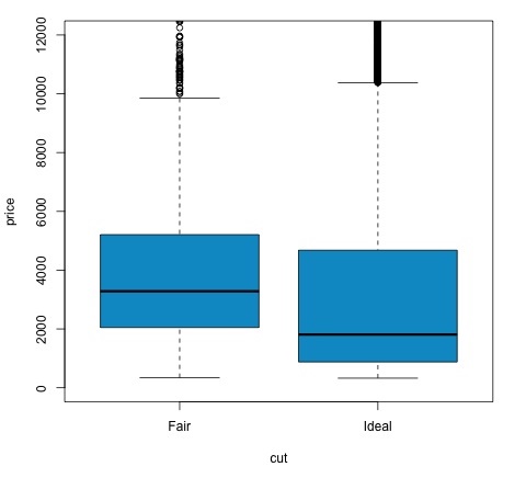
t.test(price ~ cut, data = data)

# Welch Two Sample t-test
#
# data:  price by cut
# t = 9.7484, df = 1894.8, p-value < 2.2e-16
# alternative hypothesis: true difference in means is not equal to 0
# 95 percent confidence interval:
#   719.9065 1082.5251
# sample estimates:
#   mean in group Fair mean in group Ideal
#   4358.758            3457.542

# Another way to validate the previous results is to just plot the
distributions using a box-plot
plot(price ~ cut, data = data, ylim = c(0,12000),
   col = 'deepskyblue3')
我们可以通过检查 p 值是否低于 0.05 来分析测试结果。如果是这种情况,我们保留备择假设。这意味着我们发现了两个削减因子水平之间的价格差异。根据级别的名称,我们会预期这个结果,但我们不会预期失败组中的平均价格会高于理想组中的平均价格。我们可以通过比较每个因素的均值来看到这一点。
的情节命令产生的曲线图,显示了价格和切变量之间的关系。这是一个箱线图;我们已经在 16.0.1 节中介绍了这个图,但它基本上显示了我们正在分析的两个切割水平的价格变量的分布。
方差分析
方差分析(ANOVA)是一种通过比较各组的均值和方差来分析组间分布差异的统计模型,该模型由Ronald Fisher开发。方差分析提供了几个组的均值是否相等的统计检验,因此将 t 检验推广到两个以上的组。
ANOVA 可用于比较三个或更多组的统计显着性,因为进行多个双样本 t 检验会增加发生统计 I 类错误的机会。
在提供数学解释方面,需要以下内容来理解测试。
Xij = x + (xi − x) + (xij − x)
这导致以下模型 –
Xij = μ + αi + ∈ij
其中 μ 是大均值,αi是第 i 组均值。误差项∈ij假设为正态分布的 iid。测试的零假设是 –
α1 = α2 = … = αk
在计算测试统计量方面,我们需要计算两个值 –
- 组间差异的平方和 –
$$SSD_B = \sum_{i}^{k} \sum_{j}^{n}(\bar{x_{\bar{i}}} – \bar{x})^2$$
- 组内平方和
$$SSD_W = \sum_{i}^{k} \sum_{j}^{n}(\bar{x_{\bar{ij}}} – \bar{x_{\bar{i}}})^ 2$$
固态硬盘在哪里B 具有 k−1 和 SSD 的自由度W具有 N−k 的自由度。然后我们可以定义每个度量的均方差。
小姐B = 固态硬盘B / (k – 1)
小姐w = 固态硬盘w / (N – k)
最后,ANOVA中的检验统计量定义为上述两个量的比值
F = MSB / 小姐w
它遵循具有k-1和N-k自由度的F 分布。如果原假设为真,则 F 可能接近 1。否则,组间均方 MSB 可能很大,从而导致 F 值很大。
基本上,方差分析会检查总方差的两个来源,并查看哪一部分贡献更大。这就是为什么它被称为方差分析,尽管其目的是比较组均值。
在计算统计量方面,在 R 中实际上相当简单。以下示例将演示如何完成并绘制结果。
library(ggplot2)
# We will be using the mtcars dataset

head(mtcars)
#                    mpg  cyl disp  hp drat  wt  qsec   vs am  gear carb
# Mazda RX4         21.0   6  160 110 3.90 2.620 16.46  0  1    4    4
# Mazda RX4 Wag     21.0   6  160 110 3.90 2.875 17.02  0  1    4    4
# Datsun 710        22.8   4  108  93 3.85 2.320 18.61  1  1    4    1
# Hornet 4 Drive    21.4   6  258 110 3.08 3.215 19.44  1  0    3    1
# Hornet Sportabout 18.7   8  360 175 3.15 3.440 17.02  0  0    3    2
# Valiant           18.1   6  225 105 2.76 3.460 20.22  1  0    3    1

# Let's see if there are differences between the groups of cyl in the mpg variable.
data = mtcars[, c('mpg', 'cyl')]
fit = lm(mpg ~ cyl, data = mtcars)
anova(fit)

# Analysis of Variance Table
# Response: mpg
#           Df Sum Sq Mean Sq F value    Pr(>F)
# cyl        1 817.71  817.71  79.561 6.113e-10 ***
# Residuals 30 308.33   10.28
# Signif. codes:  0 *** 0.001 ** 0.01 * 0.05 .
# Plot the distribution
plot(mpg ~ as.factor(cyl), data = mtcars, col = 'deepskyblue3')
代码将产生以下输出 –
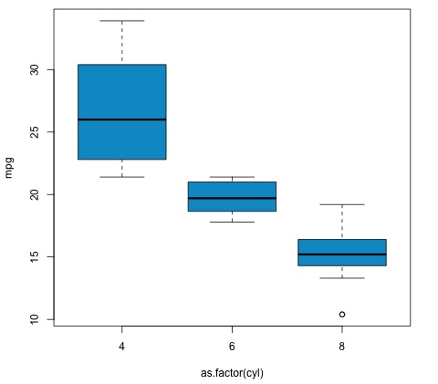
我们在示例中得到的 p 值明显小于 0.05,因此 R 返回符号“***”来表示这一点。这意味着我们拒绝原假设,并且我们发现cyl变量的不同组之间 mpg 均值之间存在差异。
